R Coding Exercise

#Load necessary packages
library(ggplot2)

Warning: package 'ggplot2' was built under R version 4.2.3

library(here)

here() starts at C:/Users/vjpan/Desktop/MADA/MADA2023/vijaypanthayi-MADA-portfolio

#Load dslabs package
library("dslabs")

#Look at help file for gapminder data
help(gapminder)

starting httpd help server ...

 done

#Get an overview of data structure
str(gapminder)

'data.frame':   10545 obs. of  9 variables:
 $ country         : Factor w/ 185 levels "Albania","Algeria",..: 1 2 3 4 5 6 7 8 9 10 ...
 $ year            : int  1960 1960 1960 1960 1960 1960 1960 1960 1960 1960 ...
 $ infant_mortality: num  115.4 148.2 208 NA 59.9 ...
 $ life_expectancy : num  62.9 47.5 36 63 65.4 ...
 $ fertility       : num  6.19 7.65 7.32 4.43 3.11 4.55 4.82 3.45 2.7 5.57 ...
 $ population      : num  1636054 11124892 5270844 54681 20619075 ...
 $ gdp             : num  NA 1.38e+10 NA NA 1.08e+11 ...
 $ continent       : Factor w/ 5 levels "Africa","Americas",..: 4 1 1 2 2 3 2 5 4 3 ...
 $ region          : Factor w/ 22 levels "Australia and New Zealand",..: 19 11 10 2 15 21 2 1 22 21 ...

#Get a summary of data
summary(gapminder)

                country           year      infant_mortality life_expectancy
 Albania            :   57   Min.   :1960   Min.   :  1.50   Min.   :13.20  
 Algeria            :   57   1st Qu.:1974   1st Qu.: 16.00   1st Qu.:57.50  
 Angola             :   57   Median :1988   Median : 41.50   Median :67.54  
 Antigua and Barbuda:   57   Mean   :1988   Mean   : 55.31   Mean   :64.81  
 Argentina          :   57   3rd Qu.:2002   3rd Qu.: 85.10   3rd Qu.:73.00  
 Armenia            :   57   Max.   :2016   Max.   :276.90   Max.   :83.90  
 (Other)            :10203                  NA's   :1453                    
   fertility       population             gdp               continent   
 Min.   :0.840   Min.   :3.124e+04   Min.   :4.040e+07   Africa  :2907  
 1st Qu.:2.200   1st Qu.:1.333e+06   1st Qu.:1.846e+09   Americas:2052  
 Median :3.750   Median :5.009e+06   Median :7.794e+09   Asia    :2679  
 Mean   :4.084   Mean   :2.701e+07   Mean   :1.480e+11   Europe  :2223  
 3rd Qu.:6.000   3rd Qu.:1.523e+07   3rd Qu.:5.540e+10   Oceania : 684  
 Max.   :9.220   Max.   :1.376e+09   Max.   :1.174e+13                  
 NA's   :187     NA's   :185         NA's   :2972                       
             region    
 Western Asia   :1026  
 Eastern Africa : 912  
 Western Africa : 912  
 Caribbean      : 741  
 South America  : 684  
 Southern Europe: 684  
 (Other)        :5586  

#Determine the type of object gapminder is
class(gapminder)

[1] "data.frame"

#Assign only countries in Africa to variable "africadata"
africadata <- subset(gapminder, continent == "Africa")

#Run the str function on the africadata dataset
str(africadata)

'data.frame':   2907 obs. of  9 variables:
 $ country         : Factor w/ 185 levels "Albania","Algeria",..: 2 3 18 22 26 27 29 31 32 33 ...
 $ year            : int  1960 1960 1960 1960 1960 1960 1960 1960 1960 1960 ...
 $ infant_mortality: num  148 208 187 116 161 ...
 $ life_expectancy : num  47.5 36 38.3 50.3 35.2 ...
 $ fertility       : num  7.65 7.32 6.28 6.62 6.29 6.95 5.65 6.89 5.84 6.25 ...
 $ population      : num  11124892 5270844 2431620 524029 4829291 ...
 $ gdp             : num  1.38e+10 NA 6.22e+08 1.24e+08 5.97e+08 ...
 $ continent       : Factor w/ 5 levels "Africa","Americas",..: 1 1 1 1 1 1 1 1 1 1 ...
 $ region          : Factor w/ 22 levels "Australia and New Zealand",..: 11 10 20 17 20 5 10 20 10 10 ...

#Run the summary function on the africadata dataset
summary(africadata)

         country          year      infant_mortality life_expectancy
 Algeria     :  57   Min.   :1960   Min.   : 11.40   Min.   :13.20  
 Angola      :  57   1st Qu.:1974   1st Qu.: 62.20   1st Qu.:48.23  
 Benin       :  57   Median :1988   Median : 93.40   Median :53.98  
 Botswana    :  57   Mean   :1988   Mean   : 95.12   Mean   :54.38  
 Burkina Faso:  57   3rd Qu.:2002   3rd Qu.:124.70   3rd Qu.:60.10  
 Burundi     :  57   Max.   :2016   Max.   :237.40   Max.   :77.60  
 (Other)     :2565                  NA's   :226                     
   fertility       population             gdp               continent   
 Min.   :1.500   Min.   :    41538   Min.   :4.659e+07   Africa  :2907  
 1st Qu.:5.160   1st Qu.:  1605232   1st Qu.:8.373e+08   Americas:   0  
 Median :6.160   Median :  5570982   Median :2.448e+09   Asia    :   0  
 Mean   :5.851   Mean   : 12235961   Mean   :9.346e+09   Europe  :   0  
 3rd Qu.:6.860   3rd Qu.: 13888152   3rd Qu.:6.552e+09   Oceania :   0  
 Max.   :8.450   Max.   :182201962   Max.   :1.935e+11                  
 NA's   :51      NA's   :51          NA's   :637                        
                       region   
 Eastern Africa           :912  
 Western Africa           :912  
 Middle Africa            :456  
 Northern Africa          :342  
 Southern Africa          :285  
 Australia and New Zealand:  0  
 (Other)                  :  0  

#Create a variable from africadata including only infant mortality and life expectancy
africadata_mort_life <- africadata[ , c("infant_mortality","life_expectancy")]

#Create a variable from africadata including only population size and life expectancy
africadata_pop_life <- africadata[ , c("population","life_expectancy")]

#Run the str function on the africadata_mort_life variable
str(africadata_mort_life)

'data.frame':   2907 obs. of  2 variables:
 $ infant_mortality: num  148 208 187 116 161 ...
 $ life_expectancy : num  47.5 36 38.3 50.3 35.2 ...

#Run the summary function on the africa_mort_life variable
summary(africadata_mort_life)

 infant_mortality life_expectancy
 Min.   : 11.40   Min.   :13.20  
 1st Qu.: 62.20   1st Qu.:48.23  
 Median : 93.40   Median :53.98  
 Mean   : 95.12   Mean   :54.38  
 3rd Qu.:124.70   3rd Qu.:60.10  
 Max.   :237.40   Max.   :77.60  
 NA's   :226                     

#Run the str function on the africadata_pop_life variable
str(africadata_pop_life)

'data.frame':   2907 obs. of  2 variables:
 $ population     : num  11124892 5270844 2431620 524029 4829291 ...
 $ life_expectancy: num  47.5 36 38.3 50.3 35.2 ...

#Run the summary function on the africadata_pop_life variable
summary(africadata_pop_life)

   population        life_expectancy
 Min.   :    41538   Min.   :13.20  
 1st Qu.:  1605232   1st Qu.:48.23  
 Median :  5570982   Median :53.98  
 Mean   : 12235961   Mean   :54.38  
 3rd Qu.: 13888152   3rd Qu.:60.10  
 Max.   :182201962   Max.   :77.60  
 NA's   :51                         

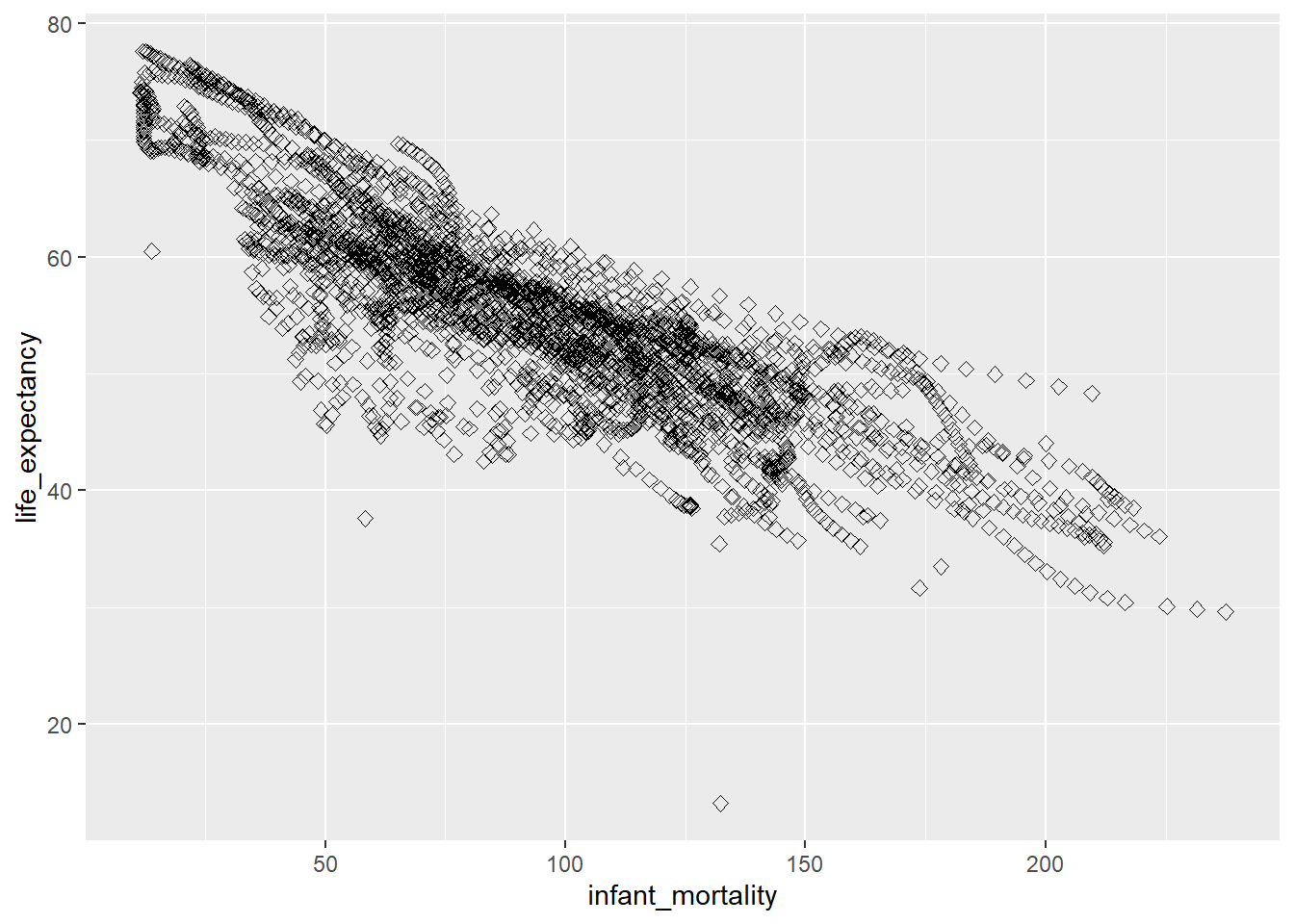
#Create a plot of life expectancy as a function of infant mortality (plot data as points)
ggplot(data=africadata_mort_life, aes(x=infant_mortality, y=life_expectancy)) +geom_point(size=2, shape=23)

Warning: Removed 226 rows containing missing values (`geom_point()`).

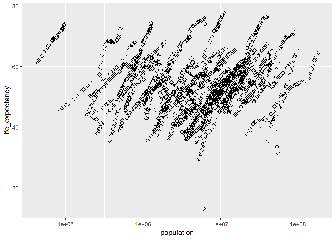
#Create a plot of population size (log) as a function of infant mortality (plot data as points)
ggplot(data=africadata_pop_life,aes(x=population, y=life_expectancy)) +geom_point(size=2, shape=23)+scale_x_log10("population")

Warning: Removed 51 rows containing missing values (`geom_point()`).

#Determine which years in the dataset have missing values
africadata_filtered <- africadata[is.na(africadata$infant_mortality),]
africadata_missing <- unique(africadata_filtered$year)
print(africadata_missing)

 [1] 1960 1961 1962 1963 1964 1965 1966 1967 1968 1969 1970 1971 1972 1973 1974
[16] 1975 1976 1977 1978 1979 1980 1981 2016

#Create a new variable with the data from africadata only including the year 2000
africadata_y2000 <- subset(africadata, year == 2000)

#Run the str function on the africadata_y2000 variable
str(africadata_y2000)

'data.frame':   51 obs. of  9 variables:
 $ country         : Factor w/ 185 levels "Albania","Algeria",..: 2 3 18 22 26 27 29 31 32 33 ...
 $ year            : int  2000 2000 2000 2000 2000 2000 2000 2000 2000 2000 ...
 $ infant_mortality: num  33.9 128.3 89.3 52.4 96.2 ...
 $ life_expectancy : num  73.3 52.3 57.2 47.6 52.6 46.7 54.3 68.4 45.3 51.5 ...
 $ fertility       : num  2.51 6.84 5.98 3.41 6.59 7.06 5.62 3.7 5.45 7.35 ...
 $ population      : num  31183658 15058638 6949366 1736579 11607944 ...
 $ gdp             : num  5.48e+10 9.13e+09 2.25e+09 5.63e+09 2.61e+09 ...
 $ continent       : Factor w/ 5 levels "Africa","Americas",..: 1 1 1 1 1 1 1 1 1 1 ...
 $ region          : Factor w/ 22 levels "Australia and New Zealand",..: 11 10 20 17 20 5 10 20 10 10 ...

#Run the summary function on the africadata_y2000 variable
summary(africadata_y2000)

         country        year      infant_mortality life_expectancy
 Algeria     : 1   Min.   :2000   Min.   : 12.30   Min.   :37.60  
 Angola      : 1   1st Qu.:2000   1st Qu.: 60.80   1st Qu.:51.75  
 Benin       : 1   Median :2000   Median : 80.30   Median :54.30  
 Botswana    : 1   Mean   :2000   Mean   : 78.93   Mean   :56.36  
 Burkina Faso: 1   3rd Qu.:2000   3rd Qu.:103.30   3rd Qu.:60.00  
 Burundi     : 1   Max.   :2000   Max.   :143.30   Max.   :75.00  
 (Other)     :45                                                  
   fertility       population             gdp               continent 
 Min.   :1.990   Min.   :    81154   Min.   :2.019e+08   Africa  :51  
 1st Qu.:4.150   1st Qu.:  2304687   1st Qu.:1.274e+09   Americas: 0  
 Median :5.550   Median :  8799165   Median :3.238e+09   Asia    : 0  
 Mean   :5.156   Mean   : 15659800   Mean   :1.155e+10   Europe  : 0  
 3rd Qu.:5.960   3rd Qu.: 17391242   3rd Qu.:8.654e+09   Oceania : 0  
 Max.   :7.730   Max.   :122876723   Max.   :1.329e+11                
                                                                      
                       region  
 Eastern Africa           :16  
 Western Africa           :16  
 Middle Africa            : 8  
 Northern Africa          : 6  
 Southern Africa          : 5  
 Australia and New Zealand: 0  
 (Other)                  : 0  

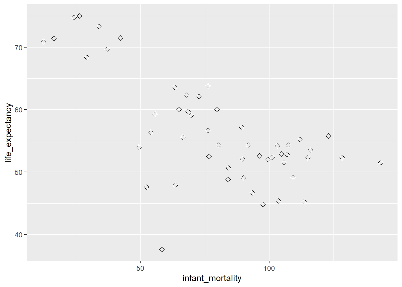
#Create a plot of life expectancy as a function of infant mortality (plot data as points) for the year 2000
ggplot(data=africadata_y2000, aes(x=infant_mortality, y=life_expectancy)) +geom_point(size=2, shape=23)

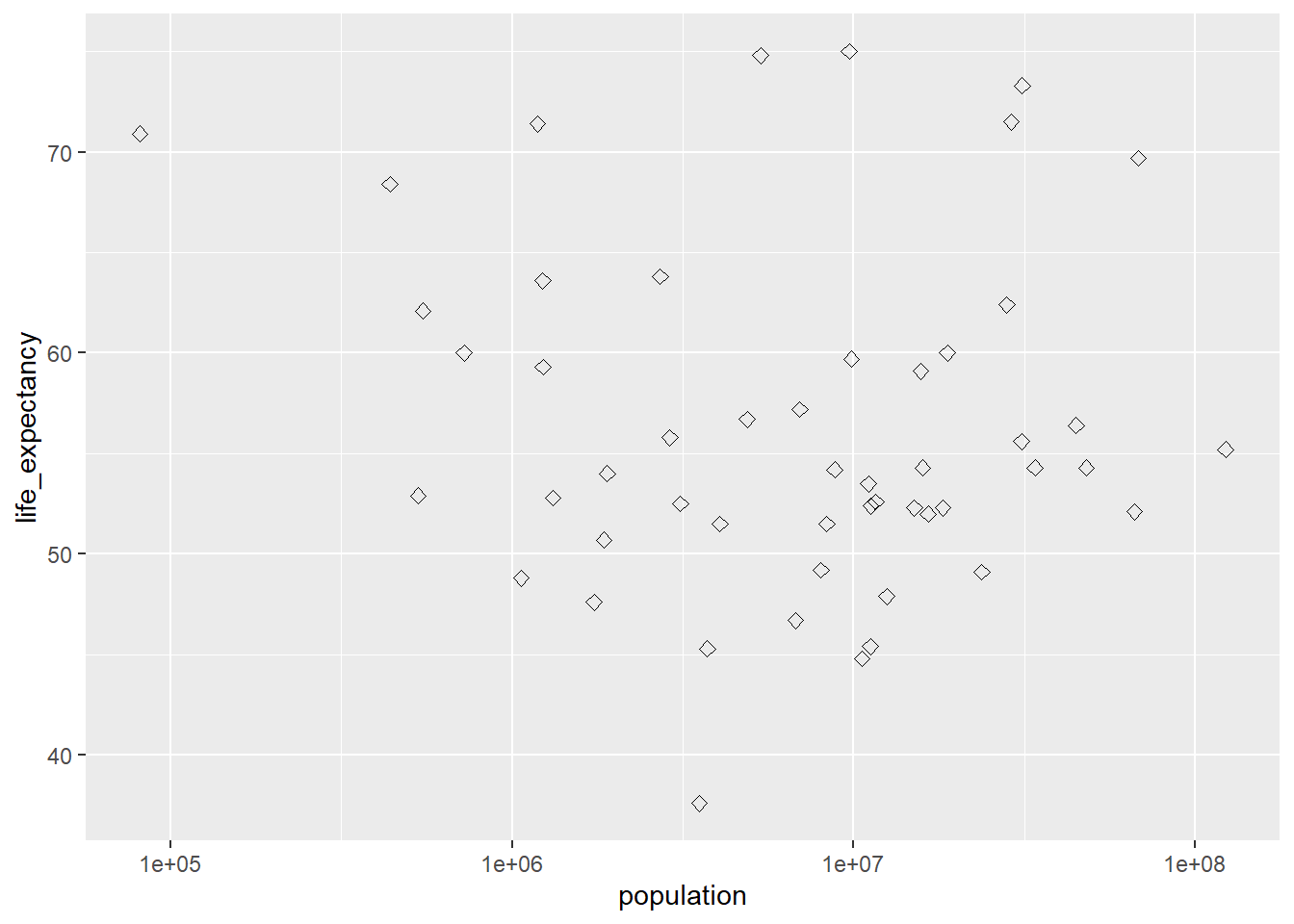
#Create a plot of population size (log) as a function of infant mortality (plot data as points) for the year 2000
ggplot(data=africadata_y2000,aes(x=population, y=life_expectancy)) +geom_point(size=2, shape=23)+scale_x_log10("population")

#Create a simple fit by setting life expectancy as the outcome and infant mortality as the predictory (using data from 2000 only)
fit1 <- lm(life_expectancy~infant_mortality, data=africadata_y2000)
summary(fit1)

Call:
lm(formula = life_expectancy ~ infant_mortality, data = africadata_y2000)

Residuals:
     Min       1Q   Median       3Q      Max 
-22.6651  -3.7087   0.9914   4.0408   8.6817 

Coefficients:
                 Estimate Std. Error t value Pr(>|t|)    
(Intercept)      71.29331    2.42611  29.386  < 2e-16 ***
infant_mortality -0.18916    0.02869  -6.594 2.83e-08 ***
---
Signif. codes:  0 '***' 0.001 '**' 0.01 '*' 0.05 '.' 0.1 ' ' 1

Residual standard error: 6.221 on 49 degrees of freedom
Multiple R-squared:  0.4701,    Adjusted R-squared:  0.4593 
F-statistic: 43.48 on 1 and 49 DF,  p-value: 2.826e-08

#Create a simple fit by setting population as the outcome and infant mortality as the predictor (using data from 2000 only)
fit2 <- lm(population~infant_mortality, data=africadata_y2000)
summary(fit2)

Call:
lm(formula = population ~ infant_mortality, data = africadata_y2000)

Residuals:
      Min        1Q    Median        3Q       Max 
-16307667 -12769228  -7828854    733380 105710100 

Coefficients:
                 Estimate Std. Error t value Pr(>|t|)
(Intercept)      12063474    8682734   1.389    0.171
infant_mortality    45564     102671   0.444    0.659

Residual standard error: 22260000 on 49 degrees of freedom
Multiple R-squared:  0.004003,  Adjusted R-squared:  -0.01632 
F-statistic: 0.1969 on 1 and 49 DF,  p-value: 0.6592

#Based on the results from the fits, it appears that infant mortality is not a good predictor of either population or life expectancy

The following added by SETH LATTNER

Based on the p-value (p=2.83e-08), I would actually conclude that infant mortality is actually a significant predictor of life expectancy.

More plotting

I want to do a little more plotting with the gapminder data for fun.

library(tidyverse)

Warning: package 'tidyverse' was built under R version 4.2.3

Warning: package 'tibble' was built under R version 4.2.3

Warning: package 'tidyr' was built under R version 4.2.3

Warning: package 'readr' was built under R version 4.2.3

Warning: package 'purrr' was built under R version 4.2.3

Warning: package 'dplyr' was built under R version 4.2.3

Warning: package 'stringr' was built under R version 4.2.3

Warning: package 'forcats' was built under R version 4.2.3

Warning: package 'lubridate' was built under R version 4.2.3

── Attaching core tidyverse packages ──────────────────────── tidyverse 2.0.0 ──
✔ dplyr     1.1.1     ✔ readr     2.1.4
✔ forcats   1.0.0     ✔ stringr   1.5.0
✔ lubridate 1.9.2     ✔ tibble    3.2.1
✔ purrr     1.0.1     ✔ tidyr     1.3.0
── Conflicts ────────────────────────────────────────── tidyverse_conflicts() ──
✖ dplyr::filter() masks stats::filter()
✖ dplyr::lag()    masks stats::lag()
ℹ Use the conflicted package (<http://conflicted.r-lib.org/>) to force all conflicts to become errors

#calculate per capita GDP
gdp_per_cap<-africadata$gdp/africadata$population
summary(gdp_per_cap)

   Min. 1st Qu.  Median    Mean 3rd Qu.    Max.    NA's 
  54.89  247.40  407.06  903.87  846.16 8527.47     637 

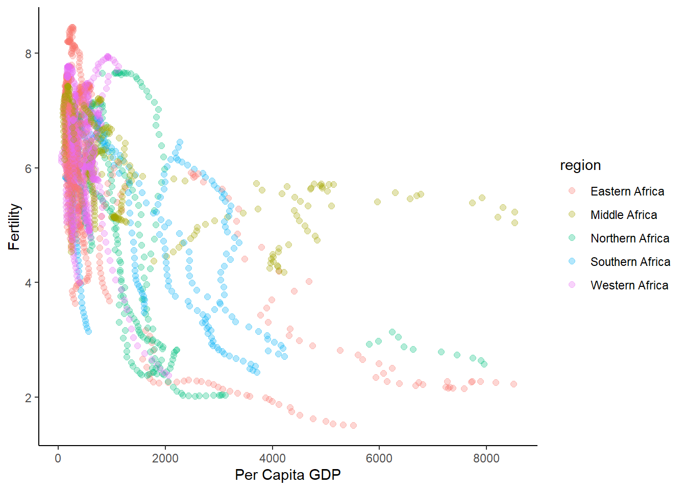
#plot fertility vs per capita GDP for each region of Africa
ggplot(africadata, aes(gdp_per_cap, fertility, color=region))+
  geom_point(cex=2, alpha=0.3)+
  xlab("Per Capita GDP")+
  ylab("Fertility")+
  theme_classic()

Warning: Removed 637 rows containing missing values (`geom_point()`).

#model fertility vs per capita GDP for each region of Africa
new_fit<-lm(fertility~gdp_per_cap+region, data=africadata)
summary(new_fit)

Call:
lm(formula = fertility ~ gdp_per_cap + region, data = africadata)

Residuals:
    Min      1Q  Median      3Q     Max 
-3.1399 -0.6288  0.0433  0.7313  3.5206 

Coefficients:
                        Estimate Std. Error t value Pr(>|t|)    
(Intercept)            6.457e+00  4.479e-02 144.164  < 2e-16 ***
gdp_per_cap           -5.914e-04  1.848e-05 -31.996  < 2e-16 ***
regionMiddle Africa    2.911e-01  7.016e-02   4.149 3.46e-05 ***
regionNorthern Africa -6.518e-01  7.804e-02  -8.352  < 2e-16 ***
regionSouthern Africa -5.947e-01  8.344e-02  -7.127 1.37e-12 ***
regionWestern Africa   1.258e-01  5.764e-02   2.182   0.0292 *  
---
Signif. codes:  0 '***' 0.001 '**' 0.01 '*' 0.05 '.' 0.1 ' ' 1

Residual standard error: 1.065 on 2264 degrees of freedom
  (637 observations deleted due to missingness)
Multiple R-squared:  0.4127,    Adjusted R-squared:  0.4114 
F-statistic: 318.2 on 5 and 2264 DF,  p-value: < 2.2e-16

table<-broom::tidy(new_fit)%>%
  knitr::kable(digits=3)
table

term	estimate	std.error	statistic	p.value
(Intercept)	6.457	0.045	144.164	0.000
gdp_per_cap	-0.001	0.000	-31.996	0.000
regionMiddle Africa	0.291	0.070	4.149	0.000
regionNorthern Africa	-0.652	0.078	-8.352	0.000
regionSouthern Africa	-0.595	0.083	-7.127	0.000
regionWestern Africa	0.126	0.058	2.182	0.029

#Based on these results, GDP is a significant predictor of fertility for each region
#of Africa. Obviously, there are many factors that would influence this, but this is
#still an informative parameter.