Flu Data Analysis

modeleval.qmd

Author

Vijay Panthayi

Model Improvement

First, lets load the necessary packages for this process

library(rsample)
library(yardstick)
library(tidymodels)
library(tidyverse)

Next, we will load the processed flu data from the processed_data folder.

flu_clean <- readRDS(here::here("fluanalysis","data","processed_data","flu_data_processed"))

Data Splitting

We’ll then need to find a way to create a testing data set from flu_clean. We will use this data to test the generated model. The rest of the data will become the training data set.

To do this, we will use set.seed() so the analysis is reproducible when random numbers are used. initial_split() will be used to split the data.

set.seed(223)
data_split <- initial_split(flu_clean,prop=3/4)
training_data <- training(data_split)
test_data <- testing(data_split)

Workflow Creation and Model Fitting

We will use tidymodels to generate our logistic regression model. We will use recipe() and worklfow() to create the workflow.

# Initiate a new recipe
logit_recipe <- recipe(Nausea ~ ., data = training_data)
# Create the logistic regression model
logistic <- logistic_reg() %>%
             set_engine("glm")
# Create the workflow
flu_wflow <- 
      workflow() %>%
      add_model(logistic) %>%
        add_recipe(logit_recipe)
flu_wflow

══ Workflow ════════════════════════════════════════════════════════════════════
Preprocessor: Recipe
Model: logistic_reg()

── Preprocessor ────────────────────────────────────────────────────────────────
0 Recipe Steps

── Model ───────────────────────────────────────────────────────────────────────
Logistic Regression Model Specification (classification)

Computational engine: glm

Model 1 Evaluation

Now that we have created the workflow, we can fit the model to the training and test data sets created previously.

training_fit <- flu_wflow %>%
                fit(data = training_data)
test_fit <- flu_wflow %>%
                fit(data = test_data)

The next step is to use the trained workflows, training_fit, to predict with unseen test data.

predict(training_fit, test_data)

Warning in predict.lm(object, newdata, se.fit, scale = 1, type = if (type == :
prediction from a rank-deficient fit may be misleading

# A tibble: 183 × 1
   .pred_class
   <fct>      
 1 No         
 2 Yes        
 3 No         
 4 No         
 5 No         
 6 Yes        
 7 No         
 8 No         
 9 No         
10 Yes        
# ℹ 173 more rows

We now want to compare the estimates. To do this, we use augment().

training_aug <- augment(training_fit, training_data)

Warning in predict.lm(object, newdata, se.fit, scale = 1, type = if (type == :
prediction from a rank-deficient fit may be misleading

Warning in predict.lm(object, newdata, se.fit, scale = 1, type = if (type == :
prediction from a rank-deficient fit may be misleading

test_aug <- augment(test_fit, test_data)

Warning in predict.lm(object, newdata, se.fit, scale = 1, type = if (type == :
prediction from a rank-deficient fit may be misleading

Warning in predict.lm(object, newdata, se.fit, scale = 1, type = if (type == :
prediction from a rank-deficient fit may be misleading

If we want to assess how well the model makes predictions, we can us an ROC curve. roc_curev() and autoplot() commands create an ROC curve which we can use to evaluate the model on the training_data and the test_data. A ROC-AUC value of 0.5 is bad, whereas a value of 1.0 is perfect. Ideally, a value greater than 0.7 is desired.

training_aug %>%
      roc_curve(truth = Nausea, .pred_No) %>%
      autoplot()

Warning: Returning more (or less) than 1 row per `summarise()` group was deprecated in
dplyr 1.1.0.
ℹ Please use `reframe()` instead.
ℹ When switching from `summarise()` to `reframe()`, remember that `reframe()`
  always returns an ungrouped data frame and adjust accordingly.
ℹ The deprecated feature was likely used in the yardstick package.
  Please report the issue at <https://github.com/tidymodels/yardstick/issues>.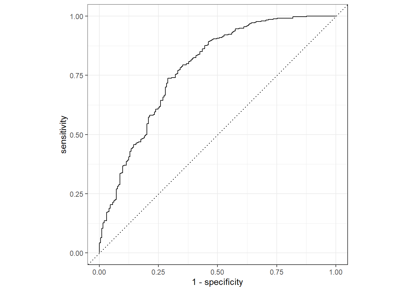

training_aug %>%
      roc_auc(truth = Nausea, .pred_No)

# A tibble: 1 × 3
  .metric .estimator .estimate
  <chr>   <chr>          <dbl>
1 roc_auc binary         0.780

Now, same for test_data.

test_aug %>%
      roc_curve(truth = Nausea, .pred_No) %>%
      autoplot()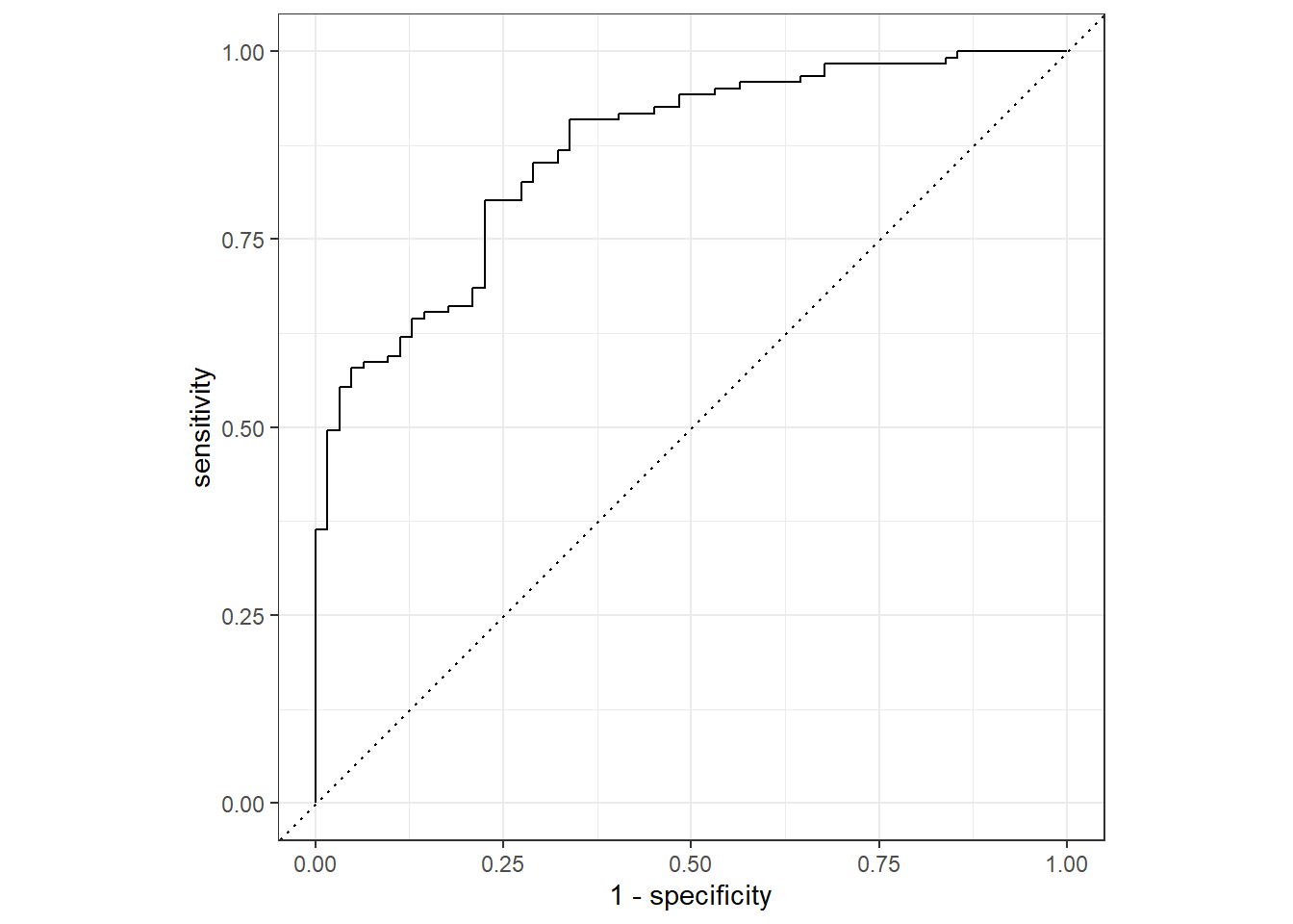

test_aug %>%
      roc_auc(truth = Nausea, .pred_No)

# A tibble: 1 × 3
  .metric .estimator .estimate
  <chr>   <chr>          <dbl>
1 roc_auc binary         0.866

The model appears to predict the data well since both the training and test data have an ROC-AUC >0.7.

Alternative Model

Now, lets repeat these steps with only 1 predictor.

logit_recipe1 <- recipe(Nausea ~ RunnyNose, data = training_data)

flu_wflow1 <- 
        workflow() %>%
        add_model(logistic) %>%
        add_recipe(logit_recipe1)

training_fit1 <- flu_wflow1 %>%
        fit(data = training_data)

test_fit1 <- flu_wflow1 %>%
        fit(data = test_data)

training_aug1 <- augment(training_fit1, training_data)
test_aug1 <- augment(test_fit1, test_data)

Lets create the ROC for the training set.

training_aug1 %>%
      roc_curve(truth = Nausea, .pred_No) %>%
      autoplot()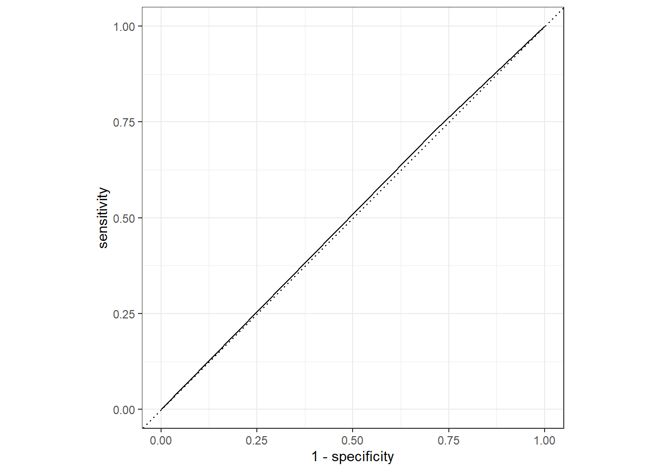

training_aug1 %>%
      roc_auc(truth = Nausea, .pred_No)

# A tibble: 1 × 3
  .metric .estimator .estimate
  <chr>   <chr>          <dbl>
1 roc_auc binary         0.507

Lets create the ROC for the test set.

test_aug1 %>%
      roc_curve(truth = Nausea, .pred_No) %>%
      autoplot()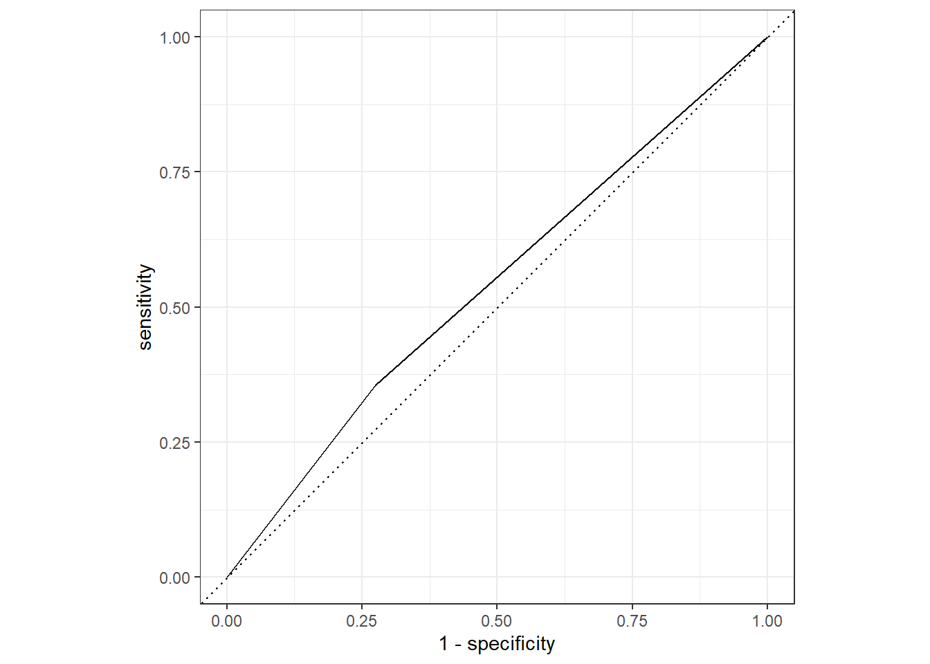

test_aug1 %>%
      roc_auc(truth = Nausea, .pred_No)

# A tibble: 1 × 3
  .metric .estimator .estimate
  <chr>   <chr>          <dbl>
1 roc_auc binary         0.541

Both ROC-AUC values were close to 0.5, which means this model is not a good fit.

Part II. Linear Regression.This section added by Betelihem G.

Data Splitting

We’ll then need to find a way to create a testing data set from flu_clean. We will use this data to test the generated model. The rest of the data will become the training data set.

To do this, we will use set.seed() so the analysis is reproducible when random numbers are used. initial_split() will be used to split the data.

set.seed(253)
data_split1 <- initial_split(flu_clean,prop=3/4)
training_data1 <- training(data_split1)
test_data1 <- testing(data_split1)

Workflow Creation and Model Fitting

We will use tidymodels to generate our logistic regression model. We will use recipe() and worklfow() to create the workflow.

# Initiate a new recipe with the continous outcome
linear_recipe <- recipe(BodyTemp ~ ., data = training_data1)
# Create the linear regression model
linear <- linear_reg() %>%
             set_engine("lm")


# Create the workflow
flu_wflow3 <- 
      workflow() %>%
      add_model(linear) %>%
        add_recipe(linear_recipe)
flu_wflow3

══ Workflow ════════════════════════════════════════════════════════════════════
Preprocessor: Recipe
Model: linear_reg()

── Preprocessor ────────────────────────────────────────────────────────────────
0 Recipe Steps

── Model ───────────────────────────────────────────────────────────────────────
Linear Regression Model Specification (regression)

Computational engine: lm

Model 1 Evaluation

Now that we have created the workflow, we can fit the model to the training and test data sets created previously.

training_fit1 <- flu_wflow3 %>%
                fit(data = training_data1)
test_fit1 <- flu_wflow3 %>%
                fit(data = test_data1)

The next step is to use the trained workflows, training_fit, to predict with unseen test data.

predict(training_fit1, test_data1)

Warning in predict.lm(object = object$fit, newdata = new_data, type =
"response"): prediction from a rank-deficient fit may be misleading

# A tibble: 183 × 1
   .pred
   <dbl>
 1 100. 
 2  99.8
 3  98.9
 4  98.7
 5  99.6
 6  99.7
 7  98.9
 8  99.6
 9  99.7
10  99.5
# ℹ 173 more rows

We now want to compare the estimates. To do this, we use augment().

training_aug3 <- augment(training_fit1, training_data1)

Warning in predict.lm(object = object$fit, newdata = new_data, type =
"response"): prediction from a rank-deficient fit may be misleading

test_aug3 <- augment(test_fit1, test_data1)

Warning in predict.lm(object = object$fit, newdata = new_data, type =
"response"): prediction from a rank-deficient fit may be misleading

test_aug3 %>%
  select(BodyTemp,.pred)

# A tibble: 183 × 2
   BodyTemp .pred
      <dbl> <dbl>
 1    102.   99.3
 2     97.9  99.6
 3     99    98.6
 4     98.1  98.7
 5     99.5  98.8
 6     98.8  98.5
 7    102.   99.2
 8    100.   99.2
 9     98.1  99.6
10     98    99.0
# ℹ 173 more rows

If we want to assess how well the model makes predictions, we can use Root Mean Square Error (RMSE)to evaluate the model on the training_data1 and the test_data1. The lower the RMSE number the better the model fit is. #for training data

training_aug3 %>%
      rmse(BodyTemp, .pred)

# A tibble: 1 × 3
  .metric .estimator .estimate
  <chr>   <chr>          <dbl>
1 rmse    standard        1.15

#Now, same for test_data.

test_aug3 %>%
      rmse(BodyTemp, .pred)

# A tibble: 1 × 3
  .metric .estimator .estimate
  <chr>   <chr>          <dbl>
1 rmse    standard       0.896

The training model RMSE is 1.15 and the test data RMSE is 0.89. These numbers tell us the difference between the predicted value and the value in the dataset. It seems both training and test models performed well.

Alternative Model with only 1 predictor

Now, lets repeat these steps with only 1 predictor.The steps are similar to the above procedure. The model type linear remains the same while the recipe changes to include only 1 predictor “RunnyNose”.

linear2 <- recipe(BodyTemp ~ RunnyNose, data = training_data1)

flu_wflow4 <- 
        workflow() %>%
        add_model(linear) %>%
        add_recipe(linear2)

training_fit2 <- flu_wflow4 %>%
        fit(data = training_data1)

test_fit2 <- flu_wflow4 %>%
        fit(data = test_data1)

training_aug4 <- augment(training_fit2, training_data1)
test_aug4 <- augment(test_fit2, test_data1)

Lets look at the RMSE for training model.

training_aug4 %>%
     select(BodyTemp, RunnyNose,.pred)

# A tibble: 547 × 3
   BodyTemp RunnyNose .pred
      <dbl> <fct>     <dbl>
 1     99.2 Yes        98.9
 2    101.  Yes        98.9
 3    101   Yes        98.9
 4     98.7 Yes        98.9
 5    102.  No         99.2
 6     97.8 Yes        98.9
 7     98.5 Yes        98.9
 8    102.  Yes        98.9
 9     98.4 Yes        98.9
10     99.3 No         99.2
# ℹ 537 more rows

training_aug4 %>%
  rmse(BodyTemp,.pred)

# A tibble: 1 × 3
  .metric .estimator .estimate
  <chr>   <chr>          <dbl>
1 rmse    standard        1.24

Calculate RMSE for testing model

test_aug4 %>%
     select(BodyTemp, RunnyNose,.pred)

# A tibble: 183 × 3
   BodyTemp RunnyNose .pred
      <dbl> <fct>     <dbl>
 1    102.  Yes        98.7
 2     97.9 No         99.0
 3     99   Yes        98.7
 4     98.1 Yes        98.7
 5     99.5 No         99.0
 6     98.8 No         99.0
 7    102.  No         99.0
 8    100.  Yes        98.7
 9     98.1 No         99.0
10     98   Yes        98.7
# ℹ 173 more rows

test_aug4 %>%
  rmse(BodyTemp,.pred)

# A tibble: 1 × 3
  .metric .estimator .estimate
  <chr>   <chr>          <dbl>
1 rmse    standard       0.986

Conclusion

Model 1 with ALL predictors

RMSE for training:1.15

RMSE for testing:0.89

Alternative model with only 1 predictor

RMSE for training:1.24

RMSE for testing:0.98

Overall, based on the RMSE values, it looks like model 1 with all predictors included is a better fit than the alternative model.